Clustering

K-means

Given $n$ observations, k-means partitions them into $k \leq n$ sets $S_1, \dots, S_k$ minimizing the within-cluster sum of squares,

\[\arg\min_S\ \sum_{i=1}^k\sum_{x \in S_i}\|x - \mu_i\|^2 = \arg\min_S\ \sum_{i=1}^k |S_i|\,\operatorname{Var}(S_i) \qquad \mu_i = \frac{1}{|S_i|}\sum_{x \in S_i}x\]

with $\mu_i$ the centroid of $S_i$. The second form says the objective is the sum of cluster variances weighted by cluster size.

Lloyd’s algorithm: alternate assignment and update until nothing moves.

Initialize $k$ centroids $m_1, \dots, m_k$.
Assignment step: attach each point to the nearest centroid,

\[S_i = \big\{x_p:\ \|x_p - m_i\|^2 \leq \|x_p - m_j\|^2 \ \ \forall j\big\}\]

Update step: recompute each centroid as the mean of its cluster,

\[m_i = \frac{1}{|S_i|}\sum_{x_j \in S_i}x_j\]

Both steps weakly decrease the objective $J$, which is bounded below by zero, and the partition space is finite (at most $k^n$ assignments), so the algorithm converges in finitely many steps. It converges to a local minimum, not the global one.

The mean is the optimal centroid: the update step is not a heuristic, it is the exact minimizer given the assignment.

Proof: With $J = \sum_{i=1}^k\sum_{x \in S_i}|x - \mu_i|^2$,

\[\frac{\partial J}{\partial\mu_i} = \frac{\partial}{\partial\mu_i}\Big[\sum_{x \in S_i}(x - \mu_i)^\top(x - \mu_i)\Big] = -2\sum_{x \in S_i}(x - \mu_i)\]

and setting this to zero,

\[\sum_{x \in S_i}(x - \mu_i) = 0 \iff \sum_{x \in S_i}x = |S_i|\,\mu_i \iff \mu_i = \frac{1}{|S_i|}\sum_{x \in S_i}x\]

Initialization: the objective is non-convex, so the starting point matters.

Random partition: assign each point to a random cluster, then compute means.
Forgy: pick $k$ random data points as the initial centroids.
Farthest point: deterministic, repeatedly take the point farthest from the current centroids.
K-means++: sample centers sequentially, each new center drawn from the remaining points with probability proportional to its squared distance to the nearest existing center,

\[m_1 \sim \mathrm{Uniform}\{x_1, \dots, x_n\} \qquad d(x_i) = \min_{j < t}\|x_i - m_j\|^2 \qquad \mathbb{P}(x_i\ \text{chosen}) = \frac{d(x_i)}{\sum_j d(x_j)}\]

This spreads the initial centers out and comes with a guarantee: the expected objective is within $O(\log k)$ of the optimum, before Lloyd’s iterations even begin.

Variants:

K-medians minimizes $\sum_i\sum_{x \in S_i}|x - \mu_i|$, using the $L_1$ norm, so the center becomes the coordinatewise median and the method is more robust to outliers.
K-medoids constrains each center to be an actual data point, which allows arbitrary distance matrices.
Fuzzy C-means is the soft version, minimizing $\sum_{i=1}^k\sum_j w_{ji}^m|x_j - \mu_i|^2$ with membership degrees

\[w_{ji} = \Bigg[\sum_{l=1}^k\bigg(\frac{\|x_j - \mu_i\|}{\|x_j - \mu_l\|}\bigg)^{\frac{2}{m-1}}\Bigg]^{-1}\]

Kernel K-means operates in an implicit feature space $\psi(x)$, allowing non-convex clusters.
Spherical K-means uses cosine similarity, normalizing the updates by $\mu_k = \big(\sum x_i\big)/|\sum x_i|$.

Computation: the distance computation vectorizes through

\[\|x_i - \mu_k\|^2 = x_i^\top x_i - 2x_i^\top\mu_k + \mu_k^\top\mu_k\]

where only the middle term is a genuine matrix product, so all pairwise squared distances follow from one matrix multiplication with no loop over observations, clusters, or dimensions. Mini-Batch K-means updates on batches of size $b$,

\[\mu_k^{\text{new}} = \mu_k + \frac{b}{v_k + b}\Big(\frac{1}{b}\sum_{i=1}^b x_i - \mu_k\Big)\]

where $v_k$ counts the points assigned to cluster $k$ so far, so the step size decays as the cluster accumulates evidence.

Failure modes:

Clusters are implicitly assumed spherical and of similar size, since the mean converges to the geometric center. Elongated, concentric, or unequal-density clusters break this.
Only convex clusters can be recovered, the boundaries being the Voronoi cells of the centroids.
Sensitive to initialization, hence to local minima; restart or use k-means++.
Sensitive to scale, so features must be standardized or high-variance features dominate the distance.
Every feature is weighted equally, and the method is sensitive to outliers and noise.
Cost is $O(n \times k \times d \times \text{iterations})$.
The curse of dimensionality: in high dimension all pairwise distances concentrate, so nearest and farthest neighbours become indistinguishable.

Hierarchical Clustering

Hierarchical clustering does not require $k$ to be fixed in advance. It produces a tree, the dendrogram, from which any number of clusters can be read off by cutting at a chosen height. It needs a dissimilarity between groups of observations, the linkage. Two directions:

Agglomerative, bottom up, repeatedly merging the pair of clusters with the smallest linkage dissimilarity;
Divisive, top down, starting from the full dataset and recursively splitting one cluster in two.

Diagram

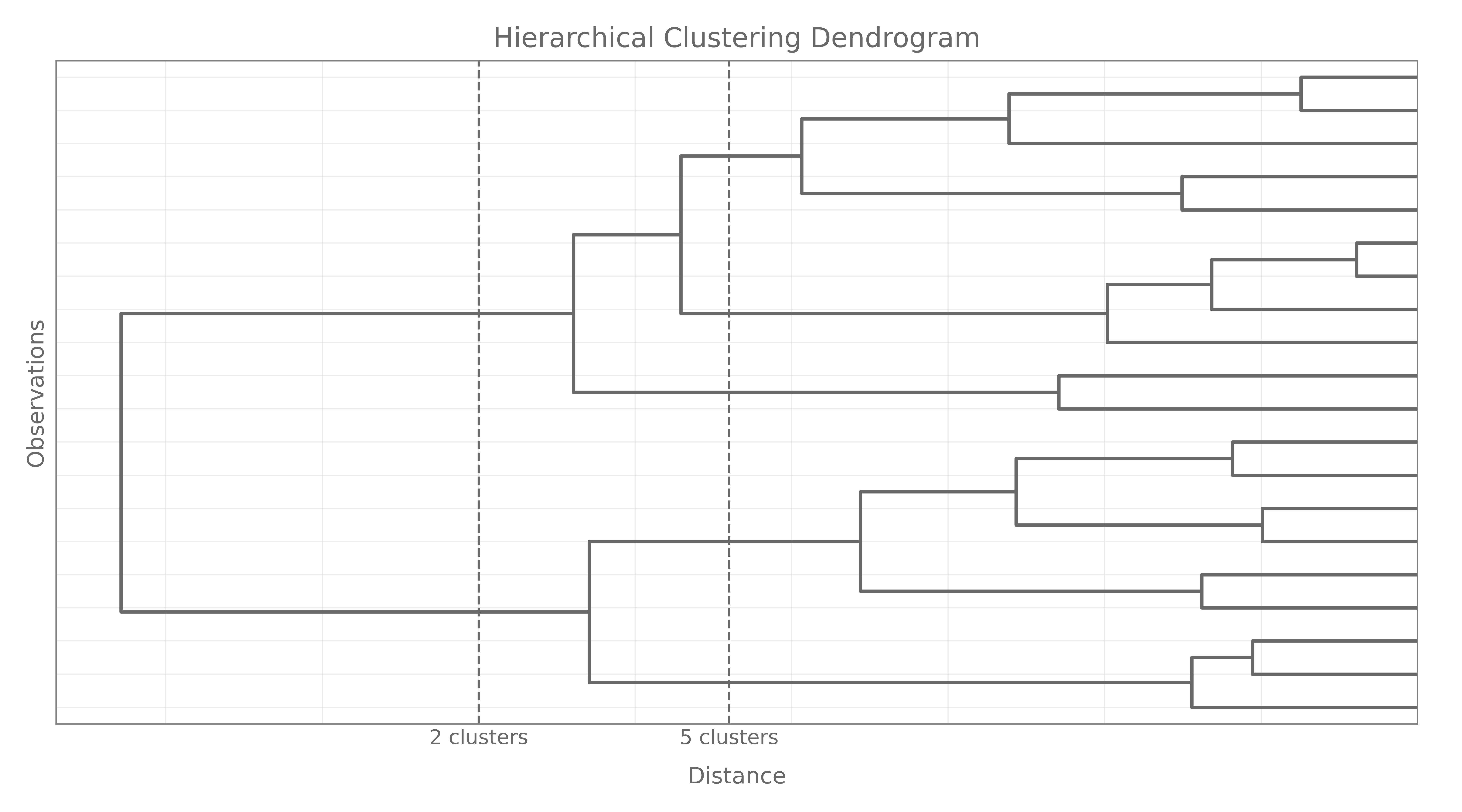
Cutting the tree at a height gives the clusters present at that dissimilarity: high cuts give few coarse clusters, low cuts give many fine ones. How well the tree actually represents the data is measured by the cophenetic correlation, the correlation between the $N(N-1)/2$ original pairwise dissimilarities $d(i,j)$ and the cophenetic dissimilarities $C(i,j)$, the heights at which $i$ and $j$ first merge.

Cluster Linkage

For clusters $A$ and $B$:

Complete (maximum): $\max_{a \in A, b \in B} d(a,b)$, giving compact clusters of similar diameter;
Single (minimum, nearest neighbour): $\min_{a \in A, b \in B} d(a,b)$, which can chain into long straggly clusters but handles non-elliptical shapes;
Average: $\dfrac{1}{|A|\,|B|}\sum_{a \in A}\sum_{b \in B}d(a,b)$, a compromise between the two;
Centroid: $d(\mu_A, \mu_B)$, which can produce inversions where a merge happens below a previous one;
Ward (minimum variance): $\dfrac{|A|\,|B|}{|A| + |B|}|\mu_A - \mu_B|^2$, the increase in within-cluster sum of squares caused by the merge, so Ward is the hierarchical analogue of the k-means objective.

Distance Functions

Minkowski: $d(x,y) = \big(\sum_i|x_i - y_i|^q\big)^{1/q}$, giving Manhattan at $q = 1$, Euclidean at $q = 2$, and Chebyshev $\max_i|x_i - y_i|$ as $q \to \infty$.
Mahalanobis: $d(x,y) = \sqrt{(x-y)^\top\Sigma^{-1}(x-y)}$, the Euclidean distance computed after whitening, so it is covariance aware and corrects for both scale and correlation. It requires estimating $\Sigma$, which is unstable and expensive in high dimension.
Cosine ($1 -$ Cosine Similarity): $d(x,y) = 1 - \dfrac{x \cdot y}{|x||y|}$, ignoring magnitude and comparing direction only, which suits high-dimensional sparse vectors.
Hamming (for Categorical Data): $d(x,y) = \sum_i\mathbf{1}(x_i \neq y_i)$.
Dynamic Time Warping (for Time Series), of possibly different lengths or speeds. Build the cost matrix $C(t_1, t_2) = d(X_{t_1}, Y_{t_2})$, then accumulate by dynamic programming,

\[D(t_1, t_2) = C(t_1, t_2) + \min\big\{D(t_1 - 1, t_2),\ D(t_1, t_2 - 1),\ D(t_1 - 1, t_2 - 1)\big\}\]

the DTW distance being the value at the final indices and the route through the table the warping path. It handles misalignment and unequal lengths, costs $O(nm)$, and is not a true metric since the triangle inequality can fail.

Metrics and Number of Clusters

Clustering Metrics

Sum-of-squares decomposition: with $\bar\mu$ the global mean,

\[\mathrm{WCSS} = \sum_{i=1}^k\sum_{x \in S_i}\|x - \mu_i\|^2 \qquad \mathrm{BCSS} = \sum_{i=1}^k|S_i|\,\|\mu_i - \bar\mu\|^2 \qquad \mathrm{TSS} = \mathrm{WCSS} + \mathrm{BCSS}\]

The total is fixed by the data, so minimizing within-cluster scatter is the same as maximizing between-cluster scatter. WCSS alone compares methods only at equal $k$, since it decreases mechanically as $k$ grows.

Silhouette (most popular internal metric): For point $i$, let $a(i)$ be its average distance to the other points in its own cluster and $b(i)$ the minimum, over other clusters, of its average distance to that cluster. Then

\[s(i) = \frac{b(i) - a(i)}{\max\{a(i), b(i)\}} \in [-1, 1] \qquad \text{score} = \frac{1}{n}\sum_i s(i)\]

Values near $1$ mean well clustered, near $0$ mean on a boundary, and negative means probably assigned to the wrong cluster. It works with any distance, but costs $O(n^2)$, is biased toward convex clusters, and is sensitive to noise.

The silhouette plot shows every point’s $s(i)$, grouped by cluster and sorted within each, which exposes structure the average hides.

Diagram

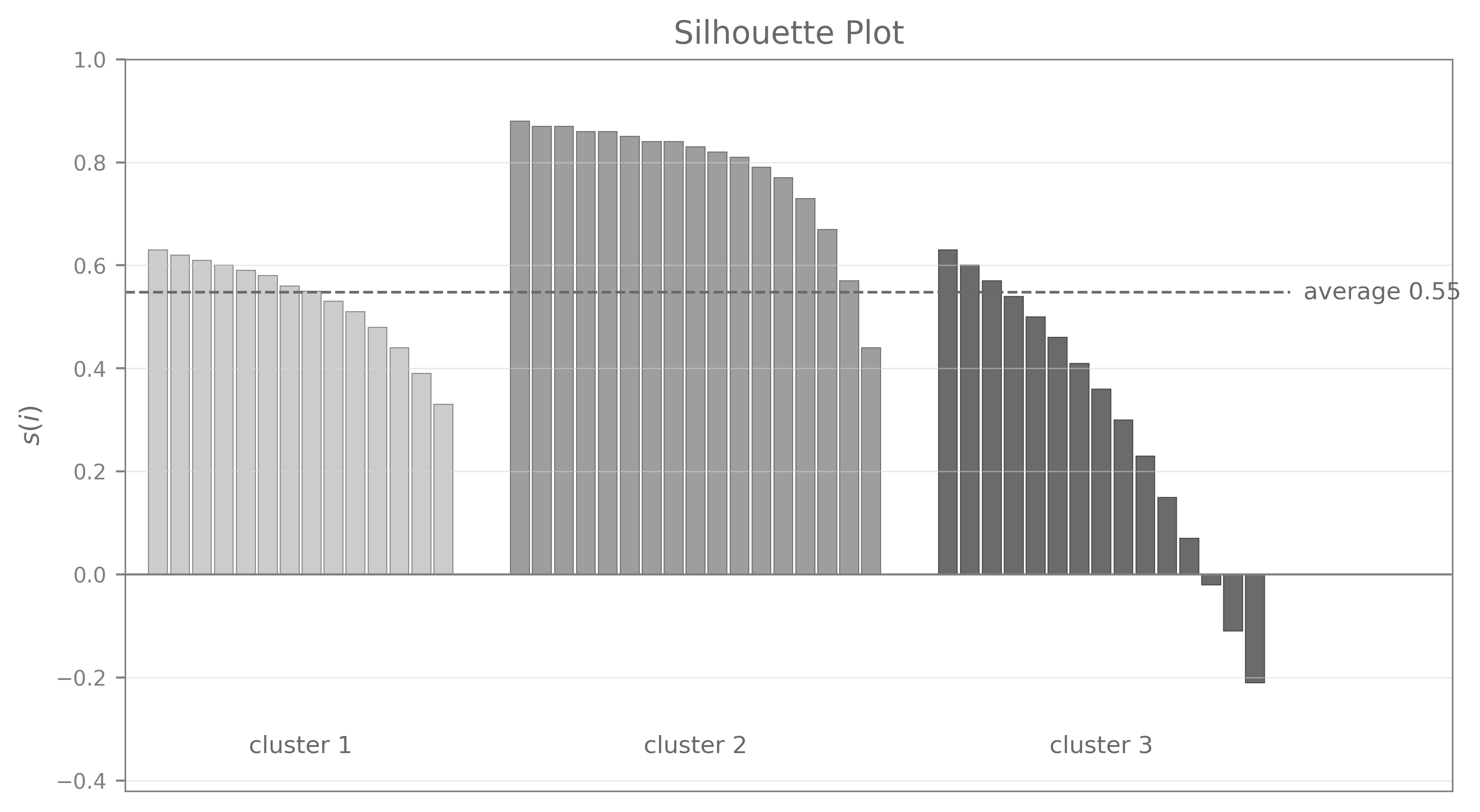
Cluster 2 is tight and well separated, sitting almost entirely above the average. Cluster 1 is acceptable but uniformly weaker. Cluster 3 has a long tail running to zero and below, so its lowest points sit closer to a neighbouring cluster than to their own and are probably misassigned. A high average silhouette can therefore coexist with one badly formed cluster, which is why the plot is read alongside the single number.

Davies–Bouldin: with $\sigma_i$ the average distance from the members of cluster $i$ to its centroid,

\[\mathrm{DB} = \frac{1}{k}\sum_{i=1}^k\max_{j \neq i}\bigg(\frac{\sigma_i + \sigma_j}{d(\mu_i, \mu_j)}\bigg)\]

The inner maximum is the worst-case similarity of cluster $i$ to any other cluster, and DB averages that worst case. The range is $[0, \infty)$ and lower is better. Costs $O(nk)$, but is biased toward spherical clusters.

Dunn:

\[D = \frac{\min_{1 \leq i < j \leq k} d(i,j)}{\max_{1 \leq c \leq k} d'(c)}\]

the smallest between-cluster distance over the largest within-cluster diameter. Range $[0, \infty)$, higher is better. Costs $O(n^2)$ and is extremely sensitive to outliers, which enter both numerator and denominator.

Choosing the Number of Clusters

Plot a criterion against $k$ and read off the turning point.

Diagram

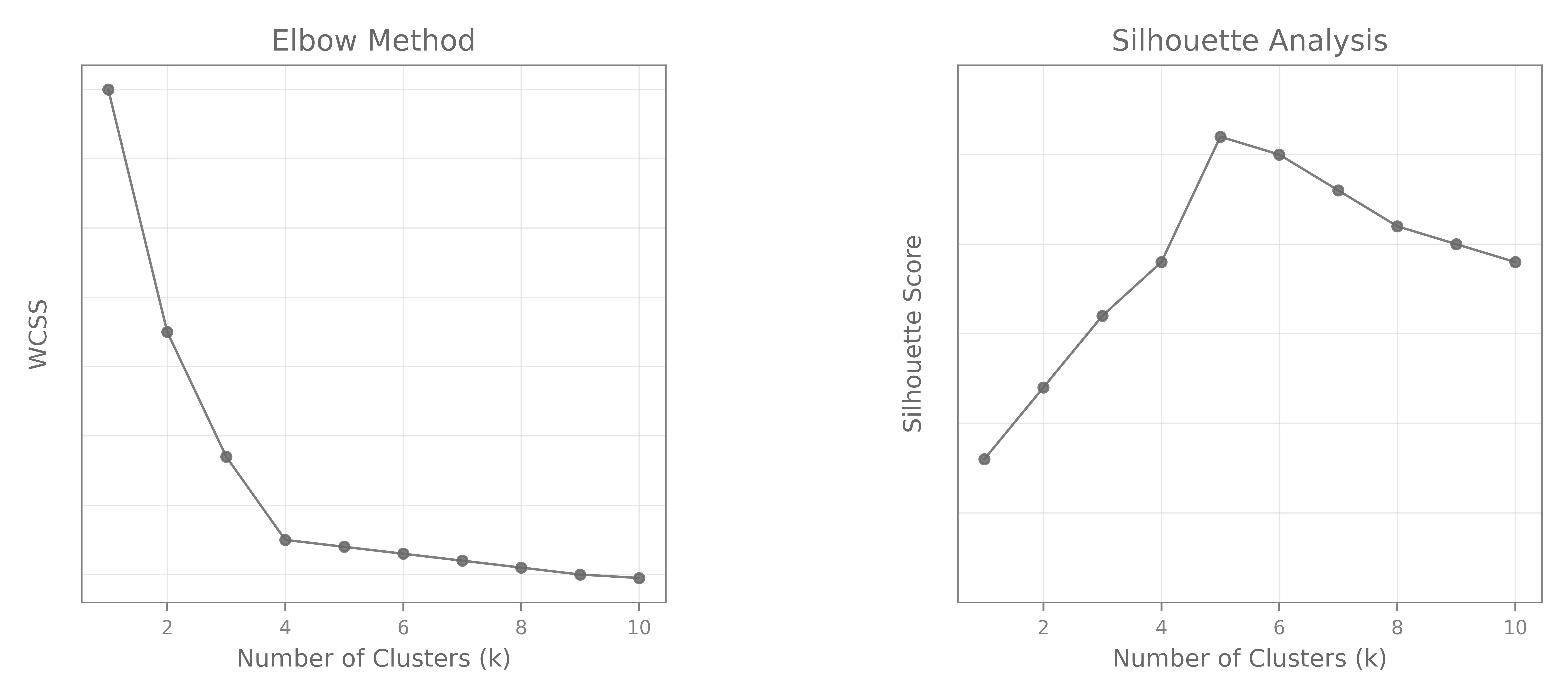
Elbow Method: compute WCSS over a range of $k$ and look for the point where the rate of decrease drops sharply. It always decreases, so the elbow rather than the minimum is the signal. It can fail when there is no clear elbow or several; the Kneedle Algorithm or a second-derivative rule automate the choice.
Silhouette Analysis: plot the silhouette score against $k$ and take the maximum. Unlike WCSS this has a genuine interior optimum.
Dendrogram: for hierarchical clustering, cut where the merge heights jump.

The two plots above are illustrative and need not agree: here the elbow suggests $k = 4$ and the silhouette $k = 5$, which is a typical amount of disagreement.

Gaussian Mixture Models

A GMM assumes the data comes from a mixture of $K$ Gaussians,

\[p(x) = \sum_{k=1}^K\pi_k\,\mathcal{N}(x \mid \mu_k, \Sigma_k) \qquad \sum_k\pi_k = 1\]

Compared to k-means it gives soft assignments (each point has a posterior probability of belonging to each component) and flexible cluster shapes, since each $\Sigma_k$ carries its own orientation and scale. The costs: it assumes Gaussianity, is sensitive to initialization, still needs $K$ specified, and has many parameters, so it is unstable in high dimension unless the covariances are constrained.

The likelihood is intractable directly:

\[L(\theta) = \prod_{i=1}^n\sum_{k=1}^K\pi_k\,\mathcal{N}(x_i \mid \mu_k, \Sigma_k) \qquad \iff \qquad \ell(\theta) = \sum_{i=1}^n\log\Big(\sum_{k=1}^K\pi_k\,\mathcal{N}(x_i \mid \mu_k, \Sigma_k)\Big)\]

The logarithm of a sum does not separate, so there is no closed-form maximizer.

Responsibilities: by Bayes, the posterior probability that component $k$ generated $x_i$ is

\[\gamma_{ik} = \mathbb{P}(z_i = k \mid x_i, \theta) = \frac{\pi_k\,\mathcal{N}(x_i \mid \mu_k, \Sigma_k)}{\sum_{j=1}^K\pi_j\,\mathcal{N}(x_i \mid \mu_j, \Sigma_j)}\]

If the latent indicators $z_{ik}$ were observed, the complete-data log-likelihood would separate,

\[\ell_c(\theta) = \sum_{i=1}^n\sum_{k=1}^K z_{ik}\big[\log\pi_k + \log\mathcal{N}(x_i \mid \mu_k, \Sigma_k)\big]\]

and EM works by maximizing its expectation instead.

Expectation Maximization

E-Step (Expectation Step): with the current parameters $\theta^{(t)}$, compute the responsibilities

\[\gamma_{ik}^{(t)} = \frac{\pi_k^{(t)}\,\mathcal{N}(x_i \mid \mu_k^{(t)}, \Sigma_k^{(t)})}{\sum_{j=1}^K\pi_j^{(t)}\,\mathcal{N}(x_i \mid \mu_j^{(t)}, \Sigma_j^{(t)})}\]

turning the hard latent assignments $z_{ik}$ into soft probabilities, which are exactly their conditional expectations.

M-Step (Maximization Step): treat the responsibilities as if they were correct and take the weighted maximum-likelihood estimates,

\[\pi_k^{(t+1)} = \frac{1}{n}\sum_{i=1}^n\gamma_{ik}^{(t)} \qquad \mu_k^{(t+1)} = \frac{\sum_i\gamma_{ik}^{(t)}x_i}{\sum_i\gamma_{ik}^{(t)}}\] \[\Sigma_k^{(t+1)} = \frac{\sum_i\gamma_{ik}^{(t)}\big(x_i - \mu_k^{(t+1)}\big)\big(x_i - \mu_k^{(t+1)}\big)^\top}{\sum_i\gamma_{ik}^{(t)}}\]

This maximizes the expected complete-data log-likelihood $Q(\theta \mid \theta^{(t)}) = \mathbb{E}_{z \mid X, \theta^{(t)}}[\ell_c(\theta)]$.

When I was an undergraduate student, I always found the Expectation-Maximization algorithm very unintuitive. I learned it many times, but it never stuck, because I never truly understood it. I’m still no pro of that EM procedure, but maybe this will help an unfortunate student that wished his exam was on supervised learning only.

It turns out that Lloyd’s Algorithm for K-means is the hard-assignment limit of the Expectation Maximization procedure. Actually, under certain (very strict) conditions, the two are equivalent: taking all mixing weights $\pi_k$ equal and all $\Sigma_k = \sigma^2 I$ with $\sigma^2 \to 0$, the responsibilities collapse to $0$ or $1$ and the two coincide exactly. This doesn’t help much does it?

What if I told you the E-Step was equivalent to the Assignment Step and the M-Step to the Update Step? The E-step computes membership given the current centers (the expected membership probabilities of each data point under the current parameter estimates, or centroid positions), and the M-step moves the centers given the memberships (updates the model parameters, or centroid positions, given the current cluster assignments).

Convergence:

The observed log-likelihood is non-decreasing at every iteration, so EM converges.
But only to a stationary point, which may be a local maximum or a saddle. Multiple restarts are standard.

This is all for today. Actually, this is way too much for any day.

References

The Elements of Statistical Learning: Data Mining, Inference, and Prediction. (2009)
Trevor Hastie, Robert Tibshirani, Jerome Friedman
Book

k-means++: The Advantages of Careful Seeding (2006)
David Arthur, Sergei Vassilvitskii
Paper

Maximum Likelihood from Incomplete Data via the EM Algorithm (1977)
A. P. Dempster, N. M. Laird, D. B. Rubin
Paper

The EM Algorithm and Extensions (2008)
GJ McLachlan, T Krishnan
Book