The Sharpe Ratio

Notation. Throughout, $T$ denotes the number of time-series observations and $N$ the number of assets. A single strategy has per-period return $R$ with mean $\mu = \mathbb{E}[R]$, variance $\sigma^2 = \operatorname{Var}(R)$, and higher central moments $\mu_k = \mathbb{E}[(R - \mu)^k]$. Standardized moments are $\gamma_3 = \mu_3/\sigma^3$ (skewness) and $\gamma_4 = \mu_4/\sigma^4$ (kurtosis). In the cross section, $\mu \in \mathbb{R}^N$ is the vector of expected (forecast) returns, $\Sigma \in \mathbb{R}^{N \times N}$ the return covariance, and $w \in \mathbb{R}^N$ the portfolio weights.

The Sharpe Ratio and its $t$-statistic

The estimated Sharpe ratio is the ratio of the sample mean return to the sample standard deviation,

\[\widehat{\mathrm{SR}} = \frac{\bar R}{\hat\sigma} \qquad \bar R = \frac{1}{T}\sum_{t=1}^T R_t \qquad \hat\sigma^2 = \frac{1}{T-1}\sum_{t=1}^T(R_t - \bar R)^2\]

Well, traditionally, we do $\mathrm{SR} = \frac{\mathbb{E}[R] - r}{\sigma}$ with $r$ the risk-free rate. But close enough. The truth is, the Sharpe Ratio is more of a means of comparing strategies of similar capacity rather than being a standalone metric. Without the context of the trading frequency and the capacity, a Sharpe Ratio by itself is pretty uninformative. A Sharpe Ratio of 2 for an ultra-high-frequency strategy is quite unimpressive, while it is extremely rare for a fundamental, long-term investor to maintain this performance for a significant amount of time.

Consider testing $H_0: \mu = 0$ (the true mean return is zero). The one-sample $t$-statistic is

\[t = \frac{\hat\mu - 0}{\hat\sigma/\sqrt{T}} = \sqrt{T}\,\frac{\bar R}{\hat\sigma} = \sqrt{T}\,\widehat{\mathrm{SR}}\]

1. The Sharpe ratio is a standardized $t$-statistic: up to the factor $\sqrt{T}$, testing whether a strategy makes money is testing whether its mean return is significantly different from zero.
2. Under $H_0$ and i.i.d. normal returns, $\sqrt{T}\,\widehat{\mathrm{SR}} \sim t_{T-1}$. The clean $t_{T-1}$ result holds only because returns were assumed normal. Real return series are skewed, fat-tailed, and serially dependent, so the exact distribution no longer applies, but the CLT makes it asymptotically normal.

Time Aggregation

When we talk about the Sharpe Ratio we generally mean the annualized Sharpe Ratio, which would be the SR measured on yearly returns. But we can transform the SR measured w.r.t. shorter time periods $t$ into a SR measured w.r.t. longer time periods $T$ (assuming $t$ divides $T$), so let $q = T/t$. We know that When we talk about the Sharpe Ratio we generally mean the annualized Sharpe Ratio, which would be the SR measured on yearly returns. But we can transform the SR measured w.r.t. shorter time periods $t$ into a SR measured w.r.t. longer time periods $T$ (assuming $t$ divides $T$), so let $q = T/t$. We know that

\[R_T = \sum_{i=1}^q R_t^{(i)}\]

Under the assumption of i.i.d. returns $R_t$,

\[\mathbb{E}[R_T] = q\,\mathbb{E}[R_t] \qquad \text{and} \qquad \operatorname{Var}[R_T] = q\,\operatorname{Var}[R_t]\] \[\mathrm{SR}[R_T] = \frac{q\,\mathbb{E}[R_t]}{\sqrt{q\,\operatorname{Var}[R_t]}} = \sqrt{q}\,\mathrm{SR}[R_t]\]

---

The Asymptotic Distribution of the Sharpe Ratio

We want the sampling distribution of $\widehat{\mathrm{SR}}$ without assuming normality. The result is

\[\sqrt{T}\,\big(\widehat{\mathrm{SR}} - \mathrm{SR}\big) \xrightarrow{d} \mathcal{N}(0, V) \qquad V = 1 + \tfrac{1}{2}\mathrm{SR}^2 - \gamma_3\,\mathrm{SR} + \frac{\gamma_4 - 3}{4}\,\mathrm{SR}^2\]

Proof: Stack the return and its squared deviation,

\[X_t = \begin{pmatrix} R_t \\ (R_t - \mu)^2 \end{pmatrix} \qquad \bar X = \frac{1}{T}\sum_{t=1}^T X_t = \begin{pmatrix} \bar R \\ \tfrac{1}{T}\sum_t (R_t - \mu)^2 \end{pmatrix} \qquad \mathbb{E}[X_t] = \begin{pmatrix} \mu \\ \sigma^2 \end{pmatrix}\]

The multivariate CLT gives

\[\sqrt{T}\,\big(\bar X - \mathbb{E}[X]\big) \xrightarrow{d} \mathcal{N}(0, \Omega) \qquad \Omega = \operatorname{Cov}(X_t)\]

so the asymptotic covariance we need is simply the covariance of one observation of $X_t$. Computing its three entries:

\[\begin{align*} \Omega_{11} &= \operatorname{Var}(R_t) = \sigma^2 \\ \Omega_{12} &= \operatorname{Cov}\big(R_t, (R_t - \mu)^2\big) = \mathbb{E}\big[(R_t - \mu)(R_t - \mu)^2\big] = \mathbb{E}\big[(R_t - \mu)^3\big] = \mu_3 \\ \Omega_{22} &= \operatorname{Var}\big((R_t - \mu)^2\big) = \mathbb{E}\big[(R_t - \mu)^4\big] - \Big(\mathbb{E}\big[(R_t - \mu)^2\big]\Big)^2 = \mu_4 - \sigma^4 \end{align*}\]

Hence

\[\Omega = \begin{pmatrix} \sigma^2 & \mu_3 \\ \mu_3 & \mu_4 - \sigma^4 \end{pmatrix}\]

where $\mu_3$ is the unnormalized third moment (skewness) and $\mu_4$ the unnormalized fourth moment (kurtosis). The gradient of $g(\mu, \sigma^2) = \mu/\sigma$ is

\[\nabla g = \begin{pmatrix} \dfrac{\partial g}{\partial\mu} \\[6pt] \dfrac{\partial g}{\partial\sigma^2} \end{pmatrix} = \begin{pmatrix} \dfrac{1}{\sigma} \\[8pt] -\dfrac{\mu}{2\sigma^3} \end{pmatrix}\]

By the delta method,

\[\begin{align*} V = \nabla g^\top\,\Omega\,\nabla g &= \begin{pmatrix} \dfrac{1}{\sigma} & -\dfrac{\mu}{2\sigma^3} \end{pmatrix} \begin{pmatrix} \sigma^2 & \mu_3 \\ \mu_3 & \mu_4 - \sigma^4 \end{pmatrix} \begin{pmatrix} \dfrac{1}{\sigma} \\[6pt] -\dfrac{\mu}{2\sigma^3} \end{pmatrix} \\[4pt] &= 1 - \frac{\mu\,\mu_3}{\sigma^4} + \frac{\mu^2\,(\mu_4 - \sigma^4)}{4\,\sigma^6} \end{align*}\]

Substitute the standardized quantities $\mathrm{SR} = \mu/\sigma$, $\gamma_3 = \mu_3/\sigma^3$, and $\gamma_4 = \mu_4/\sigma^4$:

\[V = 1 - \gamma_3\,\mathrm{SR} + \frac{\gamma_4 - 1}{4}\,\mathrm{SR}^2\]

Finally, splitting $\dfrac{\gamma_4 - 1}{4} = \dfrac{1}{2} + \dfrac{\gamma_4 - 3}{4}$ isolates the excess-kurtosis contribution and yields the final formula

\[V = 1 + \tfrac{1}{2}\mathrm{SR}^2 - \gamma_3\,\mathrm{SR} + \frac{\gamma_4 - 3}{4}\,\mathrm{SR}^2\]

Corollary (Normal returns): If returns are Gaussian, $\gamma_3 = 0$ and $\gamma_4 = 3$, so the skewness and excess-kurtosis terms vanish and

\[V = 1 + \tfrac{1}{2}\mathrm{SR}^2 \qquad \mathrm{SE}\big(\widehat{\mathrm{SR}}\big) = \sqrt{\frac{1 + \tfrac{1}{2}\mathrm{SR}^2}{T}}\]

Inference in Practice

The asymptotic variance above assumes i.i.d. returns. Real returns are serially dependent, so both the plug-in standard error and the moment estimates must be made robust. Three routes are used in increasing order of robustness. Bootstrapping helps manage that.

The Block Bootstrap

Resampling individual observations destroys autocorrelation. The block bootstrap resamples contiguous blocks of consecutive returns instead, preserving the short-range dependence structure. For example, with $T = 100$ one might draw $20$ blocks of length $5$ (with replacement) and concatenate them into a synthetic path of length $100$, recomputing $\widehat{\mathrm{SR}}$ on each such path. The block length trades off bias (too short fails to capture dependence) against variance (too long leaves too few distinct blocks).

The Studentized Bootstrap

The percentile bootstrap can have poor coverage, so studentizing (the bootstrap-$t$) improves it by bootstrapping an approximately pivotal quantity. The procedure:

1. On the full sample, compute $\widehat{\mathrm{SR}}$ and a standard-error estimate $\widehat{\mathrm{SE}}$ (plug-in or bootstrap).
2. For each bootstrap resample $b$, compute $\widehat{\mathrm{SR}}_b$ and $\widehat{\mathrm{SE}}_b$, and form the studentized statistic \(t_b^* = \frac{\widehat{\mathrm{SR}}_b - \widehat{\mathrm{SR}}}{\widehat{\mathrm{SE}}_b}\)
3. Take the empirical quantiles \(t^*_{\alpha/2}\) and \(t^*_{1-\alpha/2}\) of \(\{t_b^*\}\).
4. Form the confidence interval

\[\Big[\ \widehat{\mathrm{SR}} - t^*_{1-\alpha/2}\,\widehat{\mathrm{SE}}\ ,\ \ \widehat{\mathrm{SR}} - t^*_{\alpha/2}\,\widehat{\mathrm{SE}}\ \Big]\]

The subtraction of the upper quantile in the lower endpoint is deliberate: because $t^*_{\alpha/2}$ is typically negative, the second term adds to $\widehat{\mathrm{SR}}$, giving an interval that is correctly oriented and, unlike the percentile method, second-order accurate.

Hypothesis Test

Testing is carried out with the usual studentized statistic against a reference distribution (Gaussian or $t$):

\[t = \frac{\hat\theta - \theta_0}{\widehat{\mathrm{SE}}}\]

Example. Suppose $\widehat{\mathrm{SR}} = 0.8$ with $\widehat{\mathrm{SE}} = 0.15$, and we ask whether the true Sharpe ratio exceeds $\mathrm{SR}_0 = 0.5$. Then

\[t = \frac{\widehat{\mathrm{SR}} - \mathrm{SR}_0}{\widehat{\mathrm{SE}}} = \frac{0.8 - 0.5}{0.15} = \frac{0.3}{0.15} = 2\]

so under a normal reference there is roughly a $97.5\%$ level of confidence that the true Sharpe ratio lies above $0.5$.

The Information Ratio and the Fundamental Law

The information ratio is the Sharpe ratio of active (benchmark-relative) return, \(\mathrm{IR} = \mathrm{SR}_{\text{active}} = \mathrm{SR}_\alpha\). For a fully hedged portfolio active return equals total return and $\mathrm{IR} = \mathrm{SR}$.

A heuristic derivation links the information ratio to forecasting skill and breadth. Suppose there are $N_{\text{bets}}$ approximately independent bets, that positions are taken proportional to standardized forecast scores $f_i$ with unit cross-sectional variance, and that realized residual returns $r_i$ are standardized and cross-sectionally uncorrelated. Define the information coefficient as the correlation between forecast and realized return, $\mathrm{IC} = \operatorname{Cov}(f_i, r_i)$ (equal to the correlation since both are mean-zero, unit-variance). Then the active return $R = \sum_i f_i r_i$ has

\[\begin{align*} \mathbb{E}[R] &= \sum_{i=1}^{N_{\text{bets}}}\mathbb{E}[f_i r_i] = \sum_{i=1}^{N_{\text{bets}}}\operatorname{Cov}(f_i, r_i) = N_{\text{bets}}\cdot\mathrm{IC} \\ \operatorname{Var}(R) &= \operatorname{Var}\Big(\sum_i f_i r_i\Big) = \sum_{i=1}^{N_{\text{bets}}} f_i^2\,\operatorname{Var}(r_i) = \sum_{i=1}^{N_{\text{bets}}} f_i^2 = N_{\text{bets}} \end{align*}\]

using the normalizations $\operatorname{Var}(r_i) = 1$ and $\sum_i f_i^2 = N_{\text{bets}}$. Hence $\sigma(R) = \sqrt{N_{\text{bets}}}$ and

\[\mathrm{IR} = \frac{\mathbb{E}[R]}{\sigma(R)} = \frac{N_{\text{bets}}\cdot\mathrm{IC}}{\sqrt{N_{\text{bets}}}} = \mathrm{IC}\,\sqrt{N_{\text{bets}}}\]

This is the fundamental law of active management (Grinold, 1989): the information ratio is skill ($\mathrm{IC}$) times the square root of breadth. The general version also multiplies the RHS by $TC$ the Transfer Coefficient which is smaller than 1 and represents the friction of trading (i.e. transaction costs, slippage, impact and any other constraints).

---

MVO and Linear Algebra perspective

Maximizing the Sharpe Ratio

With forecasts $\mu = \mathbb{E}[R]$ and covariance $\Sigma = \operatorname{Cov}(R)$, the objective is to maximize the (ex ante) information ratio of the combined portfolio,

\[\max_w\ \frac{w^\top\mu}{\sqrt{w^\top\Sigma w}}\]

The ratio is invariant to the scale of $w$, so we may fix the denominator and solve

\[\max_w\ w^\top\mu \qquad \text{subject to} \qquad w^\top\Sigma w = 1\]

The Lagrangian is $\mathcal{L}(w, \lambda) = w^\top\mu - \tfrac{\lambda}{2}\big(w^\top\Sigma w - 1\big)$, with stationarity condition

\[\frac{\partial\mathcal{L}}{\partial w} = \mu - \lambda\,\Sigma w = 0 \qquad \Longrightarrow \qquad w = \frac{1}{\lambda}\,\Sigma^{-1}\mu\ \propto\ \Sigma^{-1}\mu\]

Coordinate change: $\Sigma^{-1}$ maps the forecast from return space to risk space. Equivalently, whiten: $\tilde r = \Sigma^{-1/2}r$, so $\operatorname{Cov}(\tilde r) = I$ and the whitened forecast is $\tilde\mu = \Sigma^{-1/2}\mu$, with optimal $\tilde w \propto \tilde\mu$. Since $w^\top r = \tilde w^\top\tilde r = \tilde w^\top\Sigma^{-1/2}r$, we have

\[w = \Sigma^{-1/2}\tilde w\ \propto\ \Sigma^{-1/2}\tilde\mu = \Sigma^{-1/2}\Sigma^{-1/2}\mu = \Sigma^{-1}\mu\]

The Generalized Rayleigh Quotient and the Maximal Sharpe Ratio

Lemma (Generalized Rayleigh quotient): Let $A$ be symmetric and $B \succ 0$. Then

\[\max_{u \neq 0}\ \frac{u^\top A u}{u^\top B u} = \lambda_{\max}\big(B^{-1}A\big)\]

attained at the eigenvector of $B^{-1}A$ associated with its largest eigenvalue.

Proposition (Maximal Squared Sharpe ratio): For $\Sigma \succ 0$ and $\mu \neq 0$,

\[\max_{w \neq 0}\ \frac{\big(w^\top\mu\big)^2}{w^\top\Sigma w} = \mu^\top\Sigma^{-1}\mu\]

attained at $w \propto \Sigma^{-1}\mu$. Equivalently, the maximal squared Sharpe ratio is $\mathrm{SR}_{\max}^2 = \mu^\top\Sigma^{-1}\mu$.

Proof: The squared Sharpe ratio is a generalized Rayleigh quotient with $A = \mu\mu^\top$ and $B = \Sigma$:

\[\mathrm{SR}^2 = \frac{(w^\top\mu)^2}{w^\top\Sigma w} = \frac{w^\top\mu\mu^\top w}{w^\top\Sigma w}\]

By the lemma its maximum is $\lambda_{\max}\big(\Sigma^{-1}\mu\mu^\top\big)$. The matrix $\Sigma^{-1}\mu\mu^\top$ has rank one, hence a single nonzero eigenvalue. Testing the candidate eigenvector $w = \Sigma^{-1}\mu$,

\[\Sigma^{-1}\mu\mu^\top\big(\Sigma^{-1}\mu\big) = \Sigma^{-1}\mu\,\underbrace{\big(\mu^\top\Sigma^{-1}\mu\big)}_{\text{scalar}} = \big(\mu^\top\Sigma^{-1}\mu\big)\,\Sigma^{-1}\mu\]

so $\Sigma^{-1}\mu$ is an eigenvector with eigenvalue $\lambda = \mu^\top\Sigma^{-1}\mu > 0$. Being the unique nonzero (hence largest) eigenvalue, it is the maximum, attained at $w \propto \Sigma^{-1}\mu$.

---

Combining Strategies

We now specialize the proposition to the exchangeable case: $N$ strategies, each with the same mean $\mu$, the same volatility $\sigma$ (hence the same standalone Sharpe ratio $s = \mu/\sigma$), and the same pairwise correlation $\rho$. The covariance is $\Sigma_{ii} = \sigma^2$ and $\Sigma_{ij} = \rho\sigma^2$ for $i \neq j$, and positive definiteness requires $-\tfrac{1}{N-1} < \rho < 1$.

The optimal portfolio is equally weighted. Because the assets are identical in mean, variance, and all pairwise correlations, the optimization is invariant under any permutation of the assets. The maximizer of a permutation-invariant problem is itself permutation-invariant, so all weights must be equal:

\[w_i = \frac{1}{N} \qquad i = 1, \dots, N\]

This lets us bypass inverting $\Sigma$ entirely and compute the Sharpe ratio of the equal-weight portfolio directly from its mean and variance.

Mean and variance of the equal-weight portfolio. The portfolio return is $R_p = \tfrac{1}{N}\sum_{i=1}^N R_i$, so

\[\mathbb{E}[R_p] = \frac{1}{N}\sum_{i=1}^N\mu = \mu\]

and, summing the $N$ diagonal terms and the $N(N-1)$ off-diagonal terms of the covariance,

\[\operatorname{Var}(R_p) = \frac{1}{N^2}\sum_{i=1}^N\sum_{j=1}^N\operatorname{Cov}(R_i, R_j) = \frac{1}{N^2}\Big[N\sigma^2 + N(N-1)\rho\sigma^2\Big] = \frac{\sigma^2}{N}\big[1 + (N-1)\rho\big]\]

Therefore the portfolio (and hence maximal) Sharpe ratio is

\[\mathrm{SR}_{\max} = \frac{\mathbb{E}[R_p]}{\sqrt{\operatorname{Var}(R_p)}} = \frac{\mu}{\sigma}\,\sqrt{\frac{N}{1 + (N-1)\rho}} = s\,\sqrt{\frac{N}{1 + (N-1)\rho}}\]

equivalently

\[\mathrm{SR}_{\max}^2 = \frac{N\,s^2}{1 + (N-1)\rho}\]

At $\rho = 0$ this is $\mathrm{SR}_{\max} = \sqrt{N}\,s$: the Sharpe Ratio scales at best with the square root of the number of strategies.

Number of effective strategies in the correlated case. If we had $N_{\text{eff}}$ independent strategies, the equal-weight portfolio volatility would be

\[\sigma_P^{\text{eff}} = \frac{\sigma}{\sqrt{N_{\text{eff}}}}\]

The actual equal-weight portfolio of $N$ correlated strategies has volatility

\[\sigma_P = \frac{\sigma}{\sqrt{N}}\,\sqrt{1 + (N-1)\rho}\]

so equating the two, $\dfrac{\sigma}{\sqrt{N_{\text{eff}}}} = \dfrac{\sigma}{\sqrt{N}}\,\sqrt{1 + (N-1)\rho}$, gives

\[N_{\text{eff}} = \frac{N}{1 + (N-1)\rho}\]

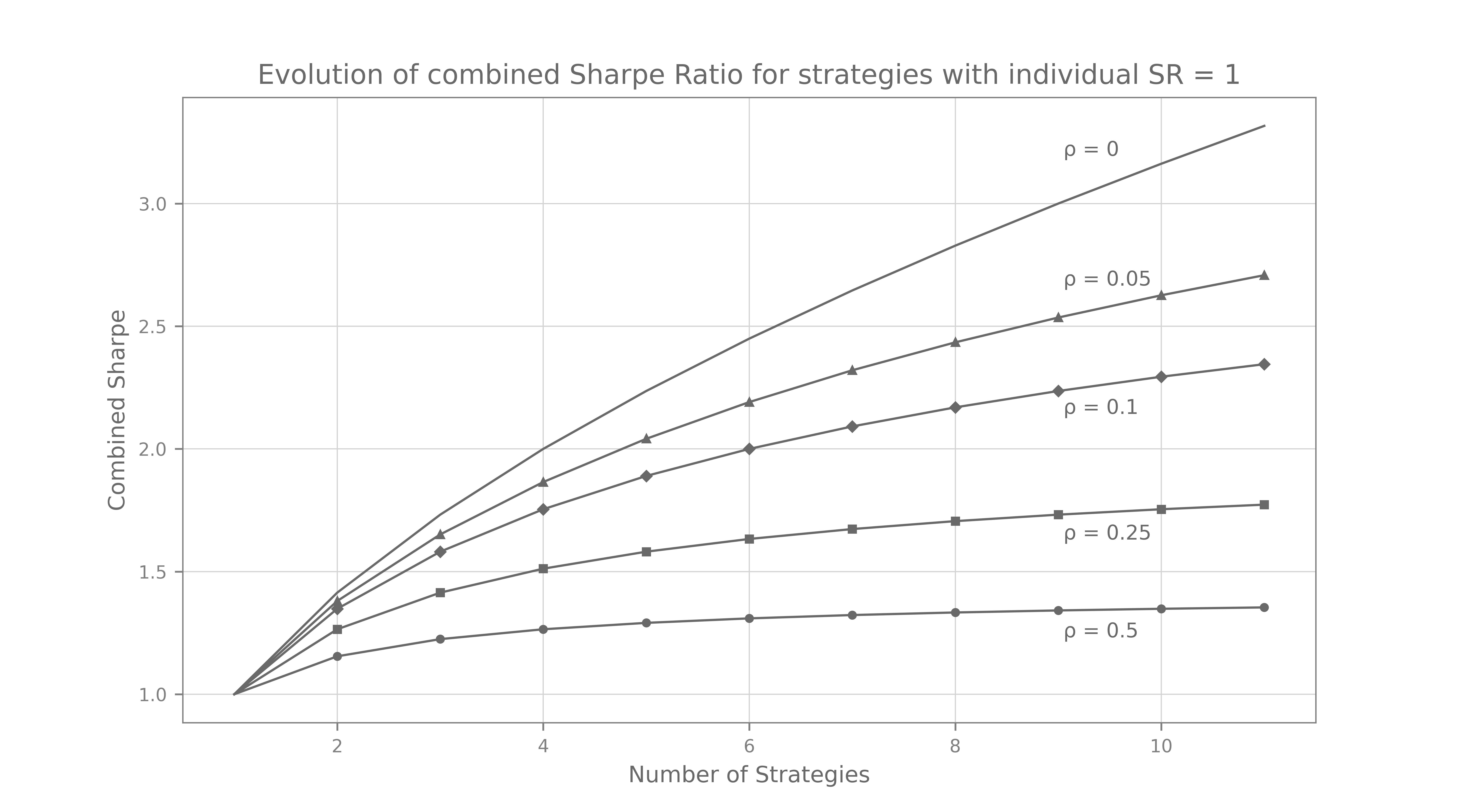
The plot above shows the evolution of the combined Sharpe of $N$ strategies all with individual Sharpe Ratio of 1. One can easily see how correlation within strategies hinders the global performance of the combined portfolio. Scalability of a hedge fund depends mostly on how uncorrelated the individual strategies are. This is why Millennium pods cannot talk to each other, by the way: to make sure that alpha doesn’t leak from one portfolio to another.

---

References

Sharpe Ratio: Estimation, Confidence Intervals, and Hypothesis Testing (2018)
Matteo Riondato, Two Sigma Investments, LP
Paper

The Statistics of Sharpe Ratios (2002)
Andrew W. Lo
Paper

Comments on the Variance of the IID estimator in Lo (2002)
Elmar Mertens
Paper

Robust performance hypothesis testing with the Sharpe ratio (2008)
Olivier Ledoit, Michael Wolf
Paper