Regularization in Regression
The Problem
Shrinkage addresses multicollinearity and performs variable selection. Eigendecompose $X^\top X = Q\Lambda Q^\top$, then $(X^\top X)^{-1} = Q\Lambda^{-1}Q^\top$, and when $X^\top X$ is near singular some eigenvalues are near zero, so the $1/\lambda_i$ blow up and $\hat\beta$ explodes. Under perfect multicollinearity $\operatorname{rank}(X^\top X) < p$, the matrix is not invertible, and OLS has no solution. Because $\operatorname{Var}(\hat\beta) = \sigma^2(X^\top X)^{-1}$ and $\operatorname{Var}(\hat y_0) = \sigma^2 x_0^\top(X^\top X)^{-1}x_0$, ill-conditioning inflates the variance of both the estimator and the forecast.
Theorem (Existence, Hoerl–Kennard): There always exists a $\lambda > 0$ for which the ridge estimator has strictly smaller mean squared error than OLS, $\mathbb{E}|\hat\beta_{\text{ridge}} - \beta|^2 < \mathbb{E}|\hat\beta_{\text{ols}} - \beta|^2$.
So regularization serves both inference (stable, interpretable coefficients) and prediction (lower out-of-sample MSE).
Ridge
General Form
Ridge adds an $L_2$ penalty,
\[\hat\beta_{\text{ridge}} = \arg\min_\beta\ \|Y - X\beta\|^2 + \lambda\|\beta\|^2 \quad \iff \quad \min_\beta\ \mathrm{RSS}\ \text{ s.t. } \textstyle\sum\beta_j^2 \leq t\]with closed form
\[\hat\beta_{\text{ridge}} = (X^\top X + \lambda I)^{-1}X^\top Y\]which exists for any $\lambda > 0$ even when $p > n$, since $\lambda I$ lifts every eigenvalue away from zero. Ridge is not scale-invariant: the OLS $\hat\beta$ are scale-equivariant (multiplying $X_j$ by $c$ rescales $\hat\beta_j$ by $1/c$) but the penalty is not, so the predictors must be standardized first. Larger $\lambda$ lowers variance and raises bias.
As SVD
Setting $X = UDV^\top$ with $U$ and $V$ orthogonal. The columns of $V$ are the right-singular vectors and eigenvectors of $X^\top X$, and the columns of $U$ are the left-singular vectors and eigenvectors of $XX^\top$. The non-zero elements of $D$ are the singular values $\sigma_i$, i.e. the square roots of the eigenvalues of $X^\top X$ (or $XX^\top$). But you already knew that, right? Right?
The OLS solution is $\hat\beta_{\text{ols}} = VD^{-1}U^\top Y = VD^+U^\top Y$, and
\[\hat\beta_{\text{ridge}} = (VD^2V^\top + \lambda I)^{-1}VDU^\top Y = V(D^2 + \lambda I)^{-1}DU^\top Y = V\operatorname{diag}\Big(\tfrac{\sigma_i}{\sigma_i^2 + \lambda}\Big)U^\top Y\]Written through the pseudoinverse, this separates the OLS part from the shrinkage filter,
\[\hat\beta_{\text{ridge}} = V\,\operatorname{diag}\Big(\tfrac{\sigma_i^2}{\sigma_i^2 + \lambda}\Big)\,D^+U^\top Y\]where $D^+U^\top Y$ is the OLS coordinate and $\tfrac{\sigma_i^2}{\sigma_i^2 + \lambda} \in (0, 1)$ is the filter. Equivalently, acting on the OLS estimate in the eigenbasis of $X^\top X$,
\[\hat\beta_{\text{ridge}} = \underbrace{V}_{\substack{\text{rotate back to}\\\text{original space}}} \ \underbrace{\operatorname{diag}\Big(\tfrac{\sigma_i^2}{\sigma_i^2 + \lambda}\Big)}_{\text{rescale eigenvalues}} \ \underbrace{V^\top}_{\substack{\text{rotate into}\\\text{eigenspace}}} \ \hat\beta_{\text{ols}}\]The filter $f_i = \sigma_i^2/(\sigma_i^2 + \lambda)$ leaves high-variance directions (large $\sigma_i$) almost untouched and drives low-variance directions toward zero, so covariates accounting for little variance shrink first.
Writing $u_i$ for the columns of $U$, the OLS fitted values are the projection of $Y$ onto the column space of $X$,
\[\hat Y_{\text{ols}} = X\hat\beta_{\text{ols}} = UDV^\top\,VD^{-1}U^\top Y = UU^\top Y = \sum_i u_i\,(u_i^\top Y)\]while ridge computes the same coordinates $u_i^\top Y$ but shrinks each one by the filter before reconstructing,
\[\hat Y_{\text{ridge}} = X\hat\beta_{\text{ridge}} = UD(D^2 + \lambda I)^{-1}DU^\top Y = \sum_i u_i\,\frac{\sigma_i^2}{\sigma_i^2 + \lambda}\,(u_i^\top Y)\]Tuning $\lambda$
The leave-one-out shortcut carries over with the ridge hat matrix $H_{\text{ridge}}(\lambda)$: the deleted residual is again the full residual inflated by one minus the leverage,
\[e_{(i)}(\lambda) = \frac{e_i(\lambda)}{1 - h_{ii}(\lambda)}\]so the leave-one-out MSE is read off a single fit at each $\lambda$,
\[\mathrm{CV}(\lambda) = \frac{1}{n}\sum_i\Big(\frac{e_i(\lambda)}{1 - h_{ii}(\lambda)}\Big)^2\]and generalized cross-validation replaces $h_{ii}(\lambda)$ by the average $\operatorname{tr}(H_{\text{ridge}})/n$. Pick the $\lambda$ minimizing $\mathrm{CV}(\lambda)$.
Lasso
Lasso penalizes the $L_1$ norm,
\[\hat\beta_{\text{lasso}} = \arg\min_\beta\ \|Y - X\beta\|^2 + \lambda\|\beta\|_1 \quad \iff \quad \min_\beta\ \mathrm{RSS}\ \text{ s.t. } \textstyle\sum|\beta_j| \leq t\]with no closed form, since $ | \beta | $ is not differentiable at zero. Optimality is read off the subgradient of $L(\beta) = \frac{1}{2}|Y - X\beta|^2 + \lambda|\beta|_1$: at the minimum $0 \in \partial L$, so per coordinate
\[X_j^\top(X\hat\beta - Y) + \lambda s_j = 0 \qquad s_j \in \partial|\hat\beta_j|\]Case 1, $\hat\beta_j = 0$: Then $s_j \in [-1, 1]$, which is feasible iff $\big\vert X_j^\top(X\hat\beta - Y)\big\vert \leq \lambda$. So a coefficient is exactly zero when the residual correlation of feature $j$, its partial correlation after orthogonalizing out the other features, is at most $\lambda$.
Case 2, $\hat\beta_j \neq 0$: Then $s_j = \operatorname{sign}(\hat\beta_j)$, so $X_j^\top(X\hat\beta - Y) = -\lambda\operatorname{sign}(\hat\beta_j)$: the penalty gradient is $\pm\lambda$, constant regardless of the magnitude of $\beta_j$.
The penalty gradient $\partial(\lambda |\beta |) = \lambda\operatorname{sign}(\beta)$ is a flat tax of size $\lambda$ applied to the partial feature. When the partial correlation drops below $\lambda$ the coefficient is taxed to zero. In the orthonormal case $X^\top X = I$ this is exactly soft-thresholding, coordinatewise,
\[\hat\beta_{\text{lasso},j} = S_\lambda(\hat\beta_{\text{ols},j}) = \operatorname{sign}(\hat\beta_{\text{ols},j})\,\big(|\hat\beta_{\text{ols},j}| - \lambda\big)_+\]Ridge, by contrast, has gradient $2\lambda\beta_j$, proportional to the current value, so large coefficients shrink more and small ones asymptotically approach but never reach zero.
Principal Component Regression
PCR drops the ill-conditioned directions outright. Take the SVD $X = UDV^\top$, keep the $k$ components with the largest singular values, and regress $Y$ on those, discarding the rest. It is the hard-thresholding cousin of ridge: ridge multiplies direction $i$ by the smooth filter $\sigma_i^2/(\sigma_i^2 + \lambda)$, while PCR multiplies by $1$ for $i \leq k$ and $0$ for $i > k$. Since the smallest-$\sigma_i$ directions carry the largest variance inflation $1/\sigma_i^2$, removing them stabilizes the fit. Its weakness is that the components are chosen from the variance of $X$ alone, ignoring $Y$, so a low-variance direction that is highly predictive can be discarded.
Bayesian Interpretation
Ridge and Lasso are posterior modes under a Gaussian likelihood with different priors,
\[\mathbb{P}(\beta \mid X, Y) \propto \mathcal{L}(Y \mid X, \beta)\,\mathbb{P}(\beta) \qquad \mathcal{L}(Y \mid X, \beta) = \Big(\tfrac{1}{\sqrt{2\pi\sigma^2}}\Big)^n\exp\Big\{-\tfrac{1}{2\sigma^2}\textstyle\sum\varepsilon_i^2\Big\}\]
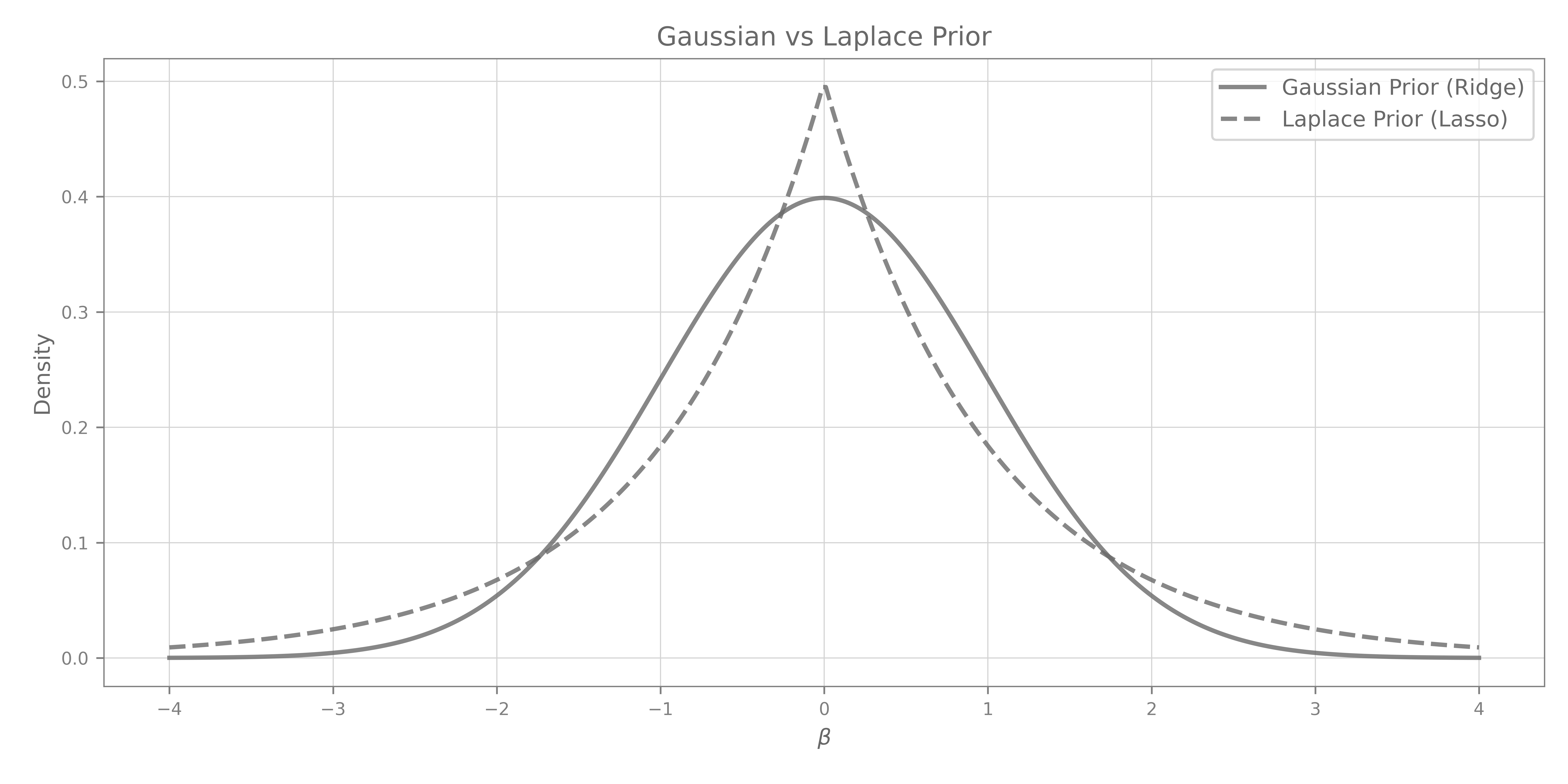
Ridge, Gaussian prior $\beta \sim \mathcal{N}(0, \tau^2)$:
\[\begin{align*} \hat\beta_{\text{ridge}} = \arg\max_\beta\ \mathbb{P}(\beta \mid X, Y) &= \arg\max_\beta\ \Big(\tfrac{1}{\sqrt{2\pi\sigma^2}}\Big)^n\exp\Big\{-\tfrac{1}{2\sigma^2}\textstyle\sum\varepsilon_i^2\Big\} \cdot \Big(\tfrac{1}{\sqrt{2\pi\tau^2}}\Big)^p\exp\Big\{-\tfrac{1}{2\tau^2}\textstyle\sum\beta_i^2\Big\} \\ &= \arg\max_\beta\ \exp\Big\{-\tfrac{1}{2\sigma^2}\textstyle\sum\varepsilon_i^2 - \tfrac{1}{2\tau^2}\textstyle\sum\beta_i^2\Big\} \\ &= \arg\min_\beta\ \Big\{\tfrac{1}{2\sigma^2}\textstyle\sum\varepsilon_i^2 + \tfrac{1}{2\tau^2}\textstyle\sum\beta_i^2\Big\} \\ &= \arg\min_\beta\ \Big\{\mathrm{RSS} + \tfrac{\sigma^2}{\tau^2}\textstyle\sum\beta_i^2\Big\} \qquad \text{which is Ridge with } \lambda = \sigma^2/\tau^2 \end{align*}\]Lasso, Laplace prior $\mathbb{P}(\beta) \propto \exp{-\textstyle\sum |\beta_i |/b}$:
\[\begin{align*} \hat\beta_{\text{lasso}} = \arg\max_\beta\ \mathbb{P}(\beta \mid X, Y) &= \arg\max_\beta\ \Big(\tfrac{1}{\sqrt{2\pi\sigma^2}}\Big)^n\exp\Big\{-\tfrac{1}{2\sigma^2}\textstyle\sum\varepsilon_i^2\Big\} \cdot \Big(\tfrac{1}{\sqrt{2b}}\Big)^p\exp\Big\{-\tfrac{1}{b}\textstyle\sum|\beta_i|\Big\} \\ &= \arg\max_\beta\ \exp\Big\{-\tfrac{1}{2\sigma^2}\textstyle\sum\varepsilon_i^2 - \tfrac{1}{b}\textstyle\sum|\beta_i|\Big\} \\ &= \arg\min_\beta\ \Big\{\tfrac{1}{2\sigma^2}\textstyle\sum\varepsilon_i^2 + \tfrac{1}{b}\textstyle\sum|\beta_i|\Big\} \\ &= \arg\min_\beta\ \Big\{\mathrm{RSS} + \tfrac{2\sigma^2}{b}\textstyle\sum|\beta_i|\Big\} \qquad \text{which is Lasso with } \lambda = 2\sigma^2/b \end{align*}\]Both are posterior modes, the ridge mode also equals the posterior mean, but the lasso mode does not.
One can easily see how the definitions of regularization as priors on the distribution of the coefficients relate to their shrinking behavior. Imagine your OLS solution $\hat\beta$ as a point on one of the two prior curves (Gaussian for Ridge, Laplace for Lasso), and the shrinking process as the effect of these priors “pulling” the estimate toward $0$. Because the Laplace prior has a sharp peak at $0$, increasing the regularization coefficient $\lambda$ can pull a coefficient exactly to $0$. In contrast, the Gaussian prior is smooth at $0$, so the corresponding Ridge penalty only shrinks coefficients continuously toward $0$ and never forces them to be exactly zero.
Lasso vs Ridge
The Grouping Effect
The grouping effect is a property of ML algorithms to put similar weights to similar features.
The Grouping Effect (Zou & Hastie, 2005): A method has the grouping effect if highly correlated predictors receive near-equal coefficients, up to sign. This is desirable for stability (small data perturbations should not flip which correlated variable is chosen), for prediction (correlated predictors jointly carry signal, so dropping one arbitrarily loses information), and for interpretability (a group of related features is included rather than an arbitrary singleton). For identical predictors $x_i = x_j$ and penalty $J$,
\[\hat\beta = \arg\min_\beta\ \|Y - X\beta\|^2 + \lambda J(\beta)\]a strictly convex $J$ forces $\hat\beta_i = \hat\beta_j$ for all $\lambda > 0$ (Lemma 2, Zou & Hastie, 2005), which ridge satisfies. Lasso ($J = |\beta|_1$) only guarantees $\hat\beta_i\hat\beta_j \geq 0$ (same sign): its solution is non-unique and it typically keeps one copy arbitrarily, with no grouping.
The effect is also quantitative. Standardize the predictors, center $Y$, and suppose $\hat\beta_i\hat\beta_j > 0$. Define the normalized coefficient gap
\[D(i,j) \triangleq \frac{\vert\hat\beta_i - \hat\beta_j\vert}{\|Y\|_1}\]Then for ridge with penalty $\lambda$ (Theorem 1 of Zou & Hastie, stated there for the $L_2$ part of the elastic net),
\[D(i,j) \leq \frac{1}{\lambda}\sqrt{2(1 - \rho)} \qquad \rho = x_i^\top x_j\]The sample correlation $\rho \to 1$ drives the bound to $0$ so highly correlated features are forced to nearly identical coefficients.
The $L_q$ Family and Sparsity
The penalty $J(\beta) = |\beta|_q^q = \sum_j |\beta_j |^q$ interpolates between these behaviours.
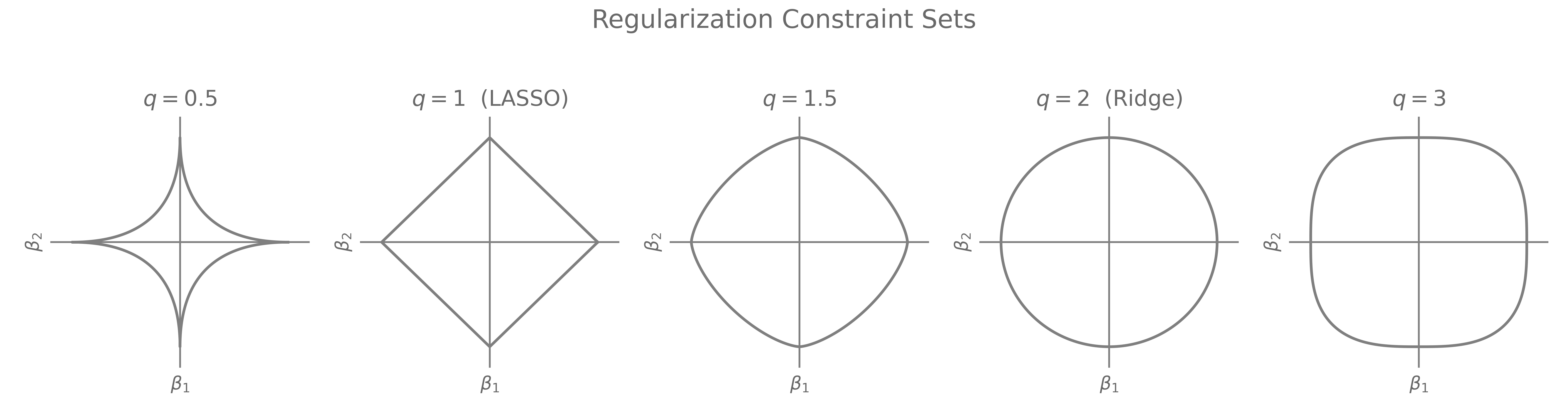
- $q = 1$ (Lasso): corners on the axes give sparsity, but it is not strictly convex, so no grouping.
- $q = 2$ (Ridge): a smooth strictly convex circle gives grouping, but has no corners, so no sparsity.
- $1 < q < 2$ (Bridge): strictly convex, so grouping but still no sparsity.
In the $L_q$ family only the Lasso ($q = 1$) produces sparse solutions (Fan & Li, 2001). Sparsity needs the non-differentiable corner, grouping needs strict convexity, and only Elastic-Net, mixing $L_1$ and $L_2$, gets both. So Elastic-Net FTW.
Rotational Invariance
Rotational Invariance (Ng, 2004): With the rotations $\mathcal{M} = {M : MM^\top = M^\top M = I,\ |M| = 1}$, an algorithm $\mathcal{L}$ is rotationally invariant if for any training set $S$, rotation $M$, and test point $x$,
\[\mathcal{L}[S](x) = \mathcal{L}[MS](Mx) \qquad MS = \{(Mx^{(i)}, y^{(i)})\}\]so predictions are unchanged by rotating the coordinate system. Ridge, OLS, kernel SVMs, and neural networks are rotationally invariant. Lasso, decision trees, naive Bayes, and feature-selection methods are not. The invariance has a cost in sparse problems: for any rotationally invariant $\mathcal{L}$ there exists a task whose labels depend on a single feature, $y = \mathbf{1}(x_1 \geq t)$, for which reaching error $\epsilon$ needs
\[m = \Omega(p/\epsilon)\]training examples (Ng, 2004). A problem that should be easy, one relevant feature, requires a sample growing with the full dimension $p$, so rotationally invariant algorithms are poor feature selectors when few features matter and $p \gg n$, exactly where Lasso’s non-invariance pays off.
On tabular data the coordinate axes are meaningful named features and the data is not rotated, so invariance costs nothing and ridge is entirely appropriate.
Elastic-Net
Elastic-net mixes the two penalties, selecting variables like Lasso while shrinking correlated predictors together like Ridge:
\[\hat\beta_{\text{EN}} = \arg\min_\beta\ \mathrm{RSS} + \lambda\sum_j\big(\alpha\,\beta_j^2 + (1 - \alpha)\,|\beta_j|\big)\]where $\alpha \in [0, 1]$ is the $L_2$ fraction ($\alpha = 1$ ridge, $\alpha = 0$ lasso). Geometrically the constraint set is pointed on the axes and rounded between them:
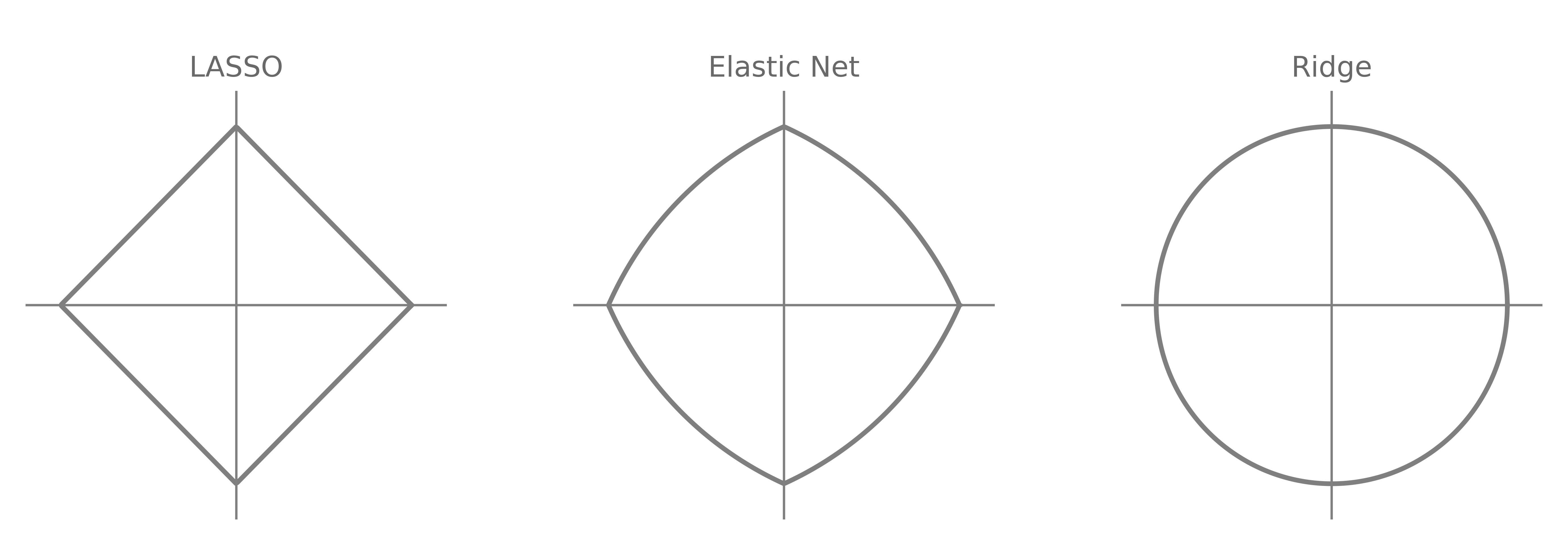
The corners on the coordinate axes give sparsity and the rounded edges spread weight across correlated predictors.
Sparsity and Rotation Together
The two are linked: rotating sparse data mixes the few informative features with much noise, which is why the rotation-invariant Ridge trails Lasso in high-sparsity regimes.
- If the important features are correlated, they combine into fewer effective features, so the problem is sparser and Lasso outperforms.
- If the noise is correlated, its dimensionality can be reduced, leaving a less sparse problem where Lasso suffers. In general Lasso loses most against Ridge moving from a sparse to a non-sparse signal, because it overshrinks small but real coefficients.
- Under general correlation across both signal and noise, Elastic-Net usually beats both.
I still use Ridge, though.
References
The Elements of Statistical Learning: Data Mining, Inference, and Prediction. (2009)
Trevor Hastie, Robert Tibshirani, Jerome Friedman
Book
Lecture notes on ridge regression (2023)
Wessel N. van Wieringen
Notes
Ridge Regression: Biased Estimation for Nonorthogonal Problems (1970)
Arthur E. Hoerl, Robert W. Kennard
Paper
Regularization and variable selection via the elastic net (2005)
Hui Zou, Trevor Hastie
Paper
Variable selection via nonconcave penalized likelihood and its oracle properties (2001)
Jianqing Fan, Runze Li
Paper
Feature selection, L1 vs. L2 regularization, and rotational invariance (2004)
Andrew Ng
Paper
Why do tree-based models still outperform deep learning on tabular data? (2022)
Léo Grinsztajn, Edouard Oyallon, Gaël Varoquaux
Paper