Tree-Based Methods
Decision Trees
A tree partitions the feature space into axis-aligned boxes $R_1, \dots, R_M$ and predicts a constant on each. The loss decomposes over regions, then over the points inside them,
\[L = \sum_{m=1}^M\sum_{i:\,x_i \in R_m}\ell\big(\hat y_m,\,y_i\big)\]where $\hat y_m$ is the within-box mean for regression or the majority class for classification. The fitted function is therefore piecewise constant.
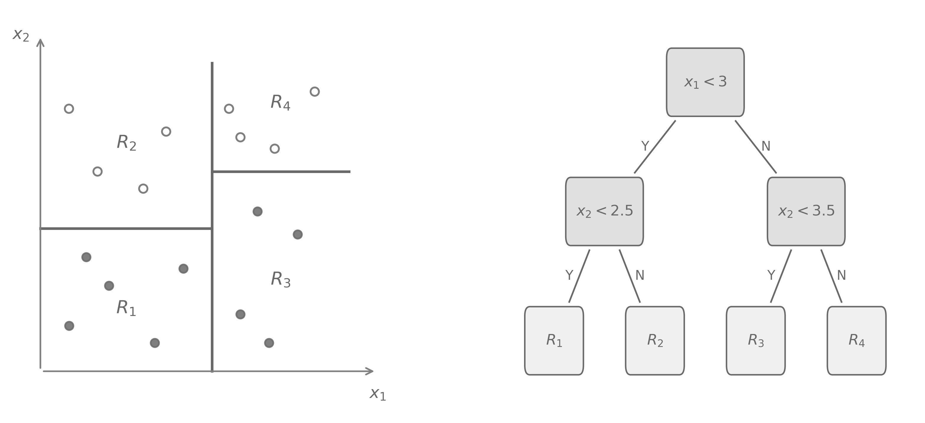
Recursive binary splitting: the tree is built greedily, since finding the optimal tree is NP-hard.
- If a stopping condition is met, make a leaf and predict the aggregate.
- Otherwise try every feature $j$ and every threshold $t$, and pick the split that reduces the loss most, equivalently the highest information gain.
- If the best gain is too small, make a leaf.
- Otherwise split the data in two and recurse on each half.
The algorithm never backtracks, which is the source of both its speed and its main weakness: a worthless split can hide an excellent one beneath it, so stopping early is dangerous. Hyperparameters controlling growth are max_depth, min_samples_leaf, min_samples_split, max_leaves, min_split_gain ($\gamma$), and min_child_weight.
Splitting criteria: impurity of a node with class proportions $p_c$,
\[\text{Gini} = 1 - \sum_c p_c^2 \qquad \qquad \text{Entropy} = -\sum_c p_c\log p_c\]and the split is chosen to maximize the information gain, the drop in impurity from parent to weighted children,
\[IG(D) = \underbrace{I(D)}_{\substack{\text{impurity}\\ \text{before the split}}} - \underbrace{\sum_{v \in \text{values}(f)}\frac{|D_v|}{|D|}\,I(D_v)}_{\substack{\text{weighted impurity}\\ \text{of the children}}}\]The above generalizes to other losses, including the traditional ones for regression, i.e. MSE, MAE, etc.
Consequences of the piecewise-constant, axis-aligned form:
- Cannot extrapolate: every prediction lies in $[\min(y), \max(y)]$ of the training data, so trees are unusable for trending series without differencing.
- Not rotationally invariant: the splits are axis-aligned, so rotating the features changes the fit. On tabular data, where the axes are meaningful named features, this is an advantage rather than a defect. I talked about this more extensively on my post on Regularization for linear models.
- Invariant to monotone transforms of a feature, since only the order of values matters for choosing a threshold. No scaling or standardization is needed.
- Excellent at interactions, since each split conditions on the previous ones, but poor at smooth linear relationships, which need a staircase of many splits to approximate.
Cost-Complexity Pruning
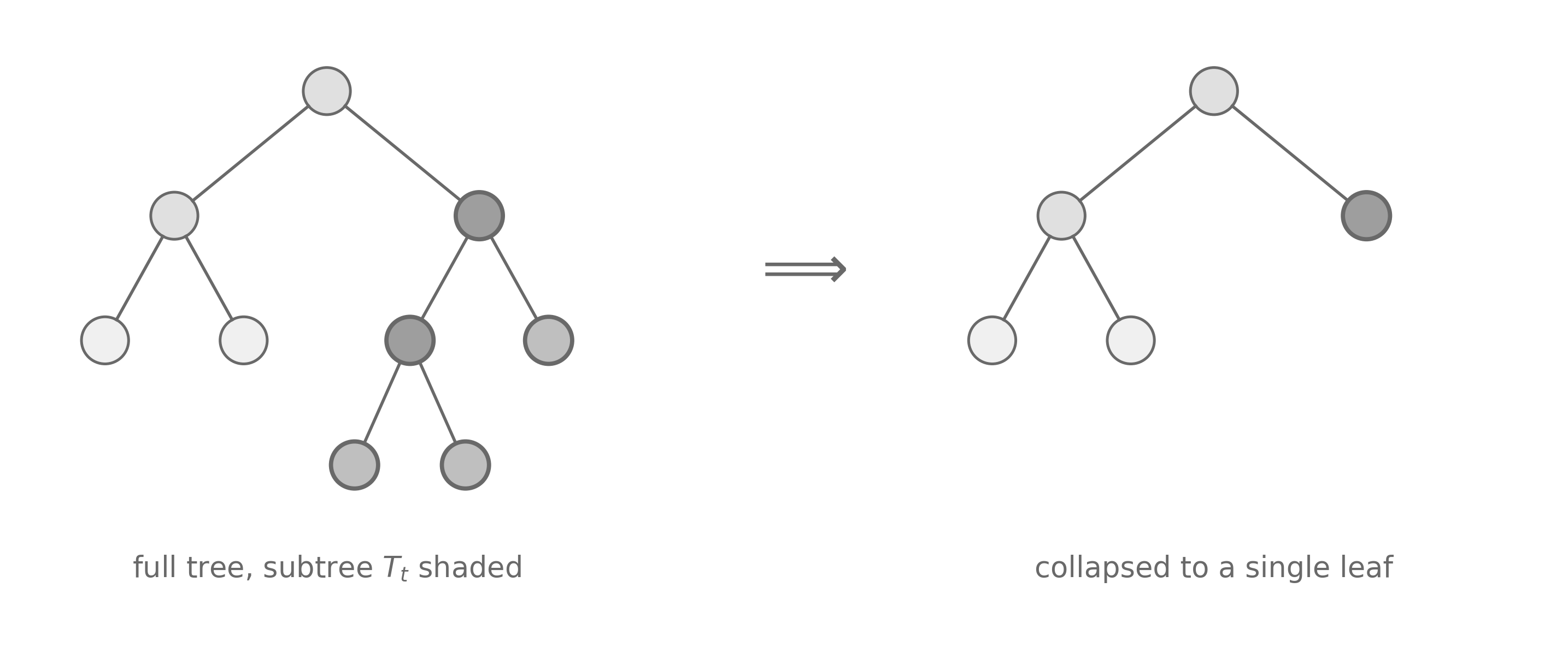
Because the algorithm is greedy, early stopping (pre-pruning) is suboptimal. A split with no immediate gain may enable a large one below it. Cross-validating every possible subtree is far too expensive. Cost-complexity pruning solves this by growing a large tree and then removing subtrees in a principled order.
For each internal node $t$, with $T_t$ the subtree rooted at $t$ and $|T_t|$ its number of leaves,
\[g_t = \frac{\overbrace{R(t)}^{\substack{\text{error at } t\\ \text{if made a leaf}}} - \overbrace{R(T_t)}^{\substack{\text{error of the}\\ \text{subtree at } t}}}{\underbrace{|T_t| - 1}_{\text{leaves removed}}}\]the error increase per leaf removed. A small $g_t$ means the subtree buys little accuracy for its complexity, so it is the weakest link and is pruned first. Pruning repeatedly gives a nested sequence
\[T_0 \supset T_1 \supset \cdots \supset T_k\]from the full tree down to a single node, and cross-validation picks among these few candidates rather than all subtrees. Along this path the implicit objective is
\[R(T) + \alpha\,|T|\]error plus a penalty per leaf, and each $g_t$ is the value of $\alpha$ at which that subtree stops paying for itself.
Random Forests
A single tree has high variance: small changes in the data produce very different trees. Random Forests fixes this by averaging many trees, and making them as uncorrelated as possible.
Bagging: for $b = 1, \dots, B$, draw a bootstrap sample of $n$ points with replacement, fit a full tree, and aggregate by averaging (regression) or majority vote (classification).
Variance of the ensemble: let each tree have variance $\sigma^2$ and pairwise correlation $\rho$. For $\bar f = \tfrac{1}{B}\sum_b f_b$,
\[\begin{align*} \operatorname{Var}(\bar f) &= \frac{1}{B^2}\Big[\sum_b\operatorname{Var}(f_b) + \sum_{b \neq b'}\operatorname{Cov}(f_b, f_{b'})\Big] \\ &= \frac{1}{B^2}\Big[B\sigma^2 + B(B-1)\rho\sigma^2\Big] = \frac{\sigma^2}{B} + \frac{B-1}{B}\rho\sigma^2 = \rho\sigma^2 + \frac{1-\rho}{B}\sigma^2 \end{align*}\]The bias is unchanged, since $\mathbb{E}[\bar f] = \mathbb{E}[f_b]$. As $B \to \infty$ the second term vanishes and the variance floors at $\rho\sigma^2$. Adding trees has diminishing returns and cannot overfit, but it also cannot push variance below the correlation floor. The only way to lower the floor is to decorrelate the trees, by
- bootstrapping the rows
- sampling the features at each split.
Feature subsampling: at each split consider only a random subset of $m$ features, with $m \approx \sqrt{p}$ for classification and $m \approx p/3$ for regression. This is what separates a random forest from plain bagged trees. Without feature subsampling, one dominant feature is chosen first by every tree and the ensemble stays correlated.
Out-of-bag estimate: the probability a given point is never drawn in $n$ draws with replacement is
\[\mathbb{P}(\text{not selected}) = \Big(1 - \frac{1}{n}\Big)^n \xrightarrow{\ n \to \infty\ } \frac{1}{e} \approx 0.368\]so each tree omits about a third of the data. Predicting each point using only the trees that did not see it gives free validation with no held-out set. This is valid only under independent sampling, so it breaks for time series.
Extremely randomized trees: draw the split threshold at random for each candidate feature rather than optimizing it. This decorrelates further and is faster, at the cost of more bias per tree.
Bagging versus boosting: bagging reduces variance by averaging many low-bias, high-variance trees fitted independently. Boosting takes the opposite view and reduces bias by fitting many high-bias, low-variance trees sequentially, each correcting the previous ones. Hence bagging uses deep trees and boosting uses shallow ones.
Gradient Boosting
Build an additive model, each term a small tree,
\[F_M(x) = F_0(x) + \nu\,h_1(x) + \nu\,h_2(x) + \cdots + \nu\,h_M(x)\]with $\nu \in (0, 1]$ the shrinkage or learning rate. You can see it resembles Gradient Descent, but in function space. Ordinary descent updates $\theta \leftarrow \theta - \eta\nabla_\theta L$, whereas here the parameter being updated is the function $F$ itself, and the step direction is the negative gradient of the loss with respect to the current predictions,
\[r_i^{(m)} = -\frac{\partial\,\ell(y_i, F)}{\partial F}\bigg|_{F = F_{m-1}(x_i)}\]For squared error $\ell = \tfrac{1}{2}(y - F)^2$ this is $r_i = y_i - F_{m-1}(x_i)$, the actual residuals. For other losses it is only the negative gradient, hence the name pseudo-residuals.
Friedman’s GBM:
- Initialize with the best constant, $F_0 = \arg\min_c\sum_i\ell(y_i, c)$.
- For $m = 1, \dots, M$:
- (a) compute the pseudo-residuals $r_i$ at the current predictions
- (b) fit a regression tree to the $r_i$, giving regions $R_{1,m}, \dots, R_{J,m}$
- (c) for each leaf, re-optimize the value against the true loss \(\gamma_{j,m} = \arg\min_\gamma\sum_{i \in R_{j,m}}\ell\big(y_i,\,F_{m-1}(x_i) + \gamma\big)\)
- (d) update $F_m(x) = F_{m-1}(x) + \nu\sum_j\gamma_{j,m}\mathbf{1}(x \in R_{j,m})$
The tree supplies the partition only, and the leaf values are then re-optimized against the actual loss. For squared error the two coincide, but for any other loss they differ. Smaller $\nu$ means smaller corrections, lower variance, and more trees needed.
Regularizing the leaf values: adding an $L_2$ penalty on the leaf weights and solving the leaf subproblem gives
\[w_j = -\frac{\overbrace{\sum_{i \in R_j}g_i}^{\text{sum of gradients}}}{\underbrace{\sum_{i \in R_j}h_i}_{\text{sum of Hessians}} + \ \lambda}\]so $L_2$ enters the denominator and shrinks every leaf value smoothly toward zero, more so for leaves holding few or low-curvature points. An $L_1$ penalty $\alpha$ instead enters the numerator as a soft threshold, $w_j = -S_\alpha\big(\sum_i g_i\big)/\big(\sum_i h_i + \lambda\big)$, which sets small leaf values exactly to zero, the same mechanism as the Lasso.
AdaBoost: gradient boosting with the exponential loss $\ell(y, F) = e^{-yF}$ for $y \in {-1, +1}$. Because the gradient of that loss is itself an exponential weight, the procedure reduces to refitting on the original data with the observations reweighted, up-weighting those currently misclassified.
XGBoost
XGboost uses the same training pseucode as Friedman but reinvents the tree-building procedure. GBM uses a first-order approximation to find the tree and then a separate line search for the leaf values. XGBoost uses a second-order expansion which unifies split finding, leaf value optimization, and regularization into one objective.
At iteration $m$ we want the tree $T_m$ minimizing $\sum_i\ell\big(y_i, F_{m-1}(x_i) + T_m(x_i)\big)$. Expanding to second order around $F_{m-1}(x_i)$,
\[\mathcal{L}^{(m)} \approx \sum_{i=1}^N\bigg[\underbrace{\ell\big(y_i, F_{m-1}(x_i)\big)}_{\text{constant, previous loss}} + \underbrace{g_i}_{\partial\ell/\partial F}T_m(x_i) + \tfrac{1}{2}\underbrace{h_i}_{\partial^2\ell/\partial F^2}T_m(x_i)^2\bigg]\]A tree is constant within each leaf, $T_m(x_i) = w_j$ for the leaf $j$ containing $i$, so the sum over observations regroups into a sum over leaves,
\[\mathcal{L}^{(m)} = \sum_{j=1}^J\bigg[\underbrace{\Big(\sum_{i \in R_j}g_i\Big)}_{G_j}w_j + \tfrac{1}{2}\underbrace{\Big(\sum_{i \in R_j}h_i\Big)}_{H_j}w_j^2\bigg] + \text{regularization}\]Adding the $L_2$ penalty $\tfrac{1}{2}\lambda\sum_j w_j^2$ on the leaf values and a fixed cost per leaf,
\[\mathcal{L}^{(m)} = \sum_{j=1}^J\Big[G_jw_j + \tfrac{1}{2}(H_j + \lambda)w_j^2\Big] + \underbrace{\gamma\,J}_{\text{penalty per leaf}}\]This is an independent quadratic in each $w_j$, so differentiating and setting to zero gives the optimal leaf value and, substituting back, the score of a node,
\[w_j^\star = -\frac{G_j}{H_j + \lambda} \qquad \text{score}(j) = -\tfrac{1}{2}\frac{G_j^2}{H_j + \lambda}\]A split is then worth making when the children score better than the parent:
\[\text{Gain} = \tfrac{1}{2}\bigg[\underbrace{\frac{G_L^2}{H_L + \lambda}}_{\text{left child score}} + \underbrace{\frac{G_R^2}{H_R + \lambda}}_{\text{right child score}} - \underbrace{\frac{G_P^2}{H_P + \lambda}}_{\text{parent score}}\bigg] - \underbrace{\gamma}_{\substack{\text{cost of}\\ \text{one more leaf}}}\]with $G_P = G_L + G_R$ and $H_P = H_L + H_R$. The $-\gamma$ makes the tree stop growing on its own, where a split whose gain does not clear the per-leaf cost is rejected, so pruning is built into the objective directly.
LightGBM
Same objective and gain formula as XGBoost, but the contributions are about speed / efficiency.
- Histogram-based splitting: bin each feature into roughly $256$ discrete buckets up front, so split finding scans bins rather than sorted values. This gives a new hyperparameter
max_bingiving the number of bins the features are bucketed into. I found it to be a great parameter to control the overall complexity of the tree, and it acts as a good regularizer. - GOSS (gradient-based one-side sampling): keep the points with large $|g_i|$, subsample the rest, and up-weight the survivors to correct the bias. Points with small gradients are already well fitted, since for squared error the gradient is the residual, so they contribute little to the next split.
- EFB (exclusive feature bundling): bundle mutually exclusive sparse features into a single feature, reducing effective dimensionality of the data.
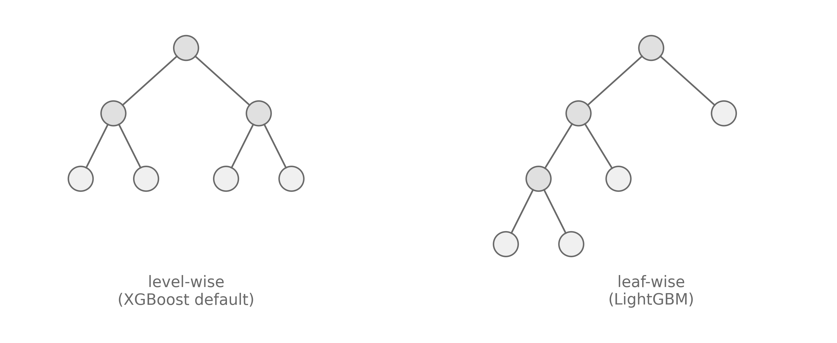
- Leaf-wise growth: always split the leaf with the highest gain anywhere in the tree, rather than completing a level first. This reaches a lower loss for the same number of leaves but produces unbalanced, deep trees and has much higher risk of overfitting.
Together these give up to an order of magnitude faster training at comparable accuracy.
Feature Importance
- Gain: total loss reduction attributable to splits on a feature. The default, but biased toward high-cardinality and continuous features, which offer more candidate thresholds.
- Split count: how often a feature is used.
- Permutation importance: shuffle one feature on held-out data and measure the drop in performance. SKlearn has an implementation.
Why Trees Still Dominate Tabular Data
These are conclusions taken directly from (Grinsztajn et al., 2022) and Makridakis’ paper on M5 competition results, that showed an overwhelming representation of LGBM in the top scorers.
- Non-smooth target functions: trees approximate jumps and thresholds naturally, whereas neural networks are biased toward smooth functions. Smoothing the target with an RBF kernel degrades boosted trees but barely affects networks, which isolates this as a real cause.
- Robustness to uninformative features: removing uninformative features narrows the gap between trees and neural networks, and adding them widens it.
- Not rotationally invariant: the axis-aligned splits exploit the fact that tabular columns are individually meaningful,.
- Mixed feature types handled natively, with no scaling, encoding, or imputation pipeline required.
- Few hyperparameters with sensible defaults, and fast training.
References
The Elements of Statistical Learning: Data Mining, Inference, and Prediction. (2009)
Trevor Hastie, Robert Tibshirani, Jerome Friedman
Book
Greedy Function Approximation: A Gradient Boosting Machine (2001)
Jerome H. Friedman
Paper
XGBoost: A Scalable Tree Boosting System (2016)
Tianqi Chen, Carlos Guestrin
Paper
LightGBM: A Highly Efficient Gradient Boosting Decision Tree (2017)
Guolin Ke, Qi Meng, Thomas Finley, Taifeng Wang, Wei Chen, Weidong Ma, Qiwei Ye, Tie-Yan Liu
Paper
CatBoost: unbiased boosting with categorical features (2018)
Liudmila Prokhorenkova, Gleb Gusev, Aleksandr Vorobev, Anna Veronika Dorogush, Andrey Gulin
Paper
Why do tree-based models still outperform deep learning on tabular data? (2022)
Léo Grinsztajn, Edouard Oyallon, Gaël Varoquaux
Paper
Feature selection, L1 vs. L2 regularization, and rotational invariance (2004)
Andrew Ng
Paper